Category: Statistics

Statistics

Why live scouting is the most important … but also why live scouts need data

We had ‘computers’ before we had digital computers, a statement that may initially sound strange but is rooted in historical fact. Long before the advent of digital computing devices, the term ‘computers’ referred to individuals—often women—tasked with performing complex mathematical calculations. These ‘female computers’ were highly intelligent and skilled women who worked on intricate mathematical problems, often aiding their male colleagues. This historical context is important as it illustrates the idea that our brains function in ways analogous to a computer, processing and interpreting data.

In fact, when dealing with uncertain situations like football, the human brain may be better equipped to compute the right answer than a digital computer. This superiority is typically found among highly intelligent individuals, or in the specific context of football, among exceptional live scouts. What distinguishes a very good live scout? A top-notch live scout possesses the ability to preview how a player will develop in the future or envision how he might perform in a different team or even in a different league. The term ‘prevision’ is chosen here deliberately, as a replacement for ‘prediction,’ in line with the philosophy of Professor Bruno de Finetti. When people use the word ‘predict,’ it can imply an ability to foretell the future with absolute certainty. Conversely, the term ‘prevision’ conveys a sense of subjectivity, emphasizing that it represents an individual’s personal anticipation of the future rather than a statement of absolute certainty.

The effectiveness of a very good live scout is rooted in his brain’s ability to absorb a wealth of data through live scouting and subsequently compute a prevision. In the case of an exceptional live scout, this prevision tends to be quite close to how reality unfolds in the future. While the very good live scout may not be right every single time, the accuracy of his previsions more often aligns with actual outcomes, demonstrating the superiority of human intuition and analysis in certain contexts.

The supremacy of live scouting stems from the human brain’s ability to process a significantly greater amount of data than current digital computers. What the brain of very good live scouts absorbs in terms of data while watching a live match far exceeds the information available in even the most detailed football statistics or what a video scout can glean from watching the same match on video. The richness and complexity of the data available in the brain of a skilled live scout make their computation of previsions a highly valuable asset. As a result, their insights and judgments often serve as the best and most essential foundation for making recruiting decisions.

Why live scouts still need data

The primary reason why live scouts continue to rely on data scouts is that data scouting enhances the efficiency of live scouting. By employing data scouting, clubs can prioritize and identify the players who are most critical to observe, streamlining the process in a way that is more efficient than relying solely on live scouts. This targeted approach ensures that live scouts focus their attention on the matches that are most important for the club. This synergy between data scouting and live scouting is well recognized, and clubs that utilize data scouting tend to employ it in this manner, maximizing the effectiveness of their scouting efforts.

What nearly all clubs overlook, however, is that data can also influence the computation that a live scout makes during live scouting, provided it is presented in a way that is actually useful to the scout. To clarify, most football data fail to assist live scouts in any meaningful way. Even the most visually appealing spider graph fails to provide any valuable insights to a live scout. However, tools like FBM charts and FBM career charts stand out as exceptions, as they can genuinely aid live scouts in understanding the players they are observing. These charts are easily interpretable once their basic principles are understood. Therefore, it is crucial to integrate data, video, and live scouting, acknowledging the unique contribution of each approach, to create a comprehensive and effective scouting strategy.

Finally, data represents another source of subjective judgments about a player, and in the context of risk management, the more varied and independent sources you have, the more robust your risk management becomes. This effectiveness stems from the fact that risk is minimized when all possible sources, provided they are independent, align with one another. When these various perspectives converge, it increases the confidence in the assessment and thereby enhances the decision-making process, reducing the likelihood of misjudgment or oversight

Why a few clubs prefer data over live scouting

Some clubs prefer data over scouting, and the most plausible explanation for this preference is that they may not have yet engaged with a very good live scout or may have had negative experiences with subpar live scouting in the past. Just as exceptional football players are rare, so too are top-tier live scouts. Therefore, it’s crucial for a club to evaluate its scouts. Interestingly, clubs that work with data often amass a considerable amount of information about football players but neglect to gather data on their own scouts. We assist clubs in implementing measuring systems that can either begin evaluating scouts from this point forward or utilize their historical scouting reports as a means to assess how well they have previewed the future of football players. This approach ensures that the evaluation process is comprehensive, taking into account both the potential of the players and the effectiveness of the scouting staff.

In conclusion, live scouting stands as the most crucial form of scouting and should serve as the decisive factor in recruiting decisions. However, to enable live scouts to arrive at more accurate previsions of the future, it’s essential to provide them with football data in a format that their brains can effectively utilize for computation. Tools like FBM charts and FBM career charts are prime examples of how data can be structured to enhance the live scouting process. By integrating these elements, clubs can create a more effective and nuanced approach to scouting that leverages the unique strengths of both live observation and data analysis.

FBM career chart Jeppe Okkels

Grading players

Grading players comes with a myriad of pitfalls. To begin with: talent is a right skewed distribution like this:

What this means is that in professional football the probability of finding a player scoring a 10 is much smaller than finding a player scoring a 1 or a 2. Yt, if you look into the player database of football clubs you almost never see the above distribution. What this means is that the scouts in that club are overestimating the players they are grading.

There are some mitigating circumstances. For instance, for most clubs it is too much work to grade players with a 1 or a 2. So they simply skip those players to save time. Skipping badly performing players is a risk though, because now it becomes harder to check whether the grades given by the scouts match this distribution. So a club that has the time and budget to also grade badly performing players really ought to do so as it is a check on the quality of their scouts. Because when you see a scout only grading players with a 7 or higher, you know that the judgment of that scout has very little value.

Football Behavior Management (FBM) stats follow the above distribution.

Relative or absolute grading?

So the second pitfall is whether you grade the player relative to his current team or the team you are scouting for, or whether you grade him with a 10 being the best player who has ever played and a 0 being the worst player ever played. Relative grading is much easier than absolute grading. But absolute grading has the advantage of being less time constrained. If you do relative grading then you ought to decide whether you grade the player for his current team (or even match) he is playing in, or whether you grade him for the team you are scouting him for, his potential future team. A player who is currently playing in an easier league with more time and space might score a high grade for his current team, but a good scout might see that he would struggle in a team in a tougher league with less time and space and for that reason give him a lower grade.

If you grade a player as he is playing in his current team or even for the actual match you are seeing, then the problem arises that it becomes much harder to compare this grade to other players graded playing for other teams in other matches. So if a club chooses this kind of grading, then they need to be very watchful of people not generalizing the same grade as meaning the same level of performance. This is very hard for people, even if they are conscious of the issue. Because if player X scores a 8 and player Y scores a 9, it is very hard for our unconsciousness to understand that player X is actually the better player as he scored the 8 in a tougher league than player Y scoring a 9.

So it is much better to grade players for the team you want them to play in in the future. But even then the grade is time constrained as the team you are scouting for might change over time. Players that scored an 8 for the first season, might be a 7 in the season thereafter and even only a 6 two seasons later as the team becomes stronger and stronger. If the club has the right infrastructure to keep track of all the judgments of players, in almost all cases, older grades are never adjusted for a team that has been developed and has become stronger. What this means is that a decision to hire a player might have been the right decision in the first season turned out to be the wrong decision in a later season because the club failed to take into account that the majority of the reports for that player were made for a time period where the team was weaker.

To avoid all of these pitfalls, FBM stats are absolute.

One number to rule them all

Modern football requires high quality decision making at high speed. In order to speed up decision making, a single grade helps a lot. Yet, a single grade can lower the quality of decision making. For a single grade a club first needs to decide how to deal with the difference between specialists and generalists. Most players are specialists. If a single grade covers every aspect of playing football, a single grade has a strong bias in favor of the few generalists. This doesn’t have to be a problem, as long as the club is aware of this bias or prefers generalists over specialists.

One can use a single grade to cover specialists. For instance if the grade is simply only for that aspect where the player excels in. For most defenders (but not all!) their single grade would reflect their ability to defend. For most strikers (but not all!) their single grade would reflect their ability to score goals. Yet, even if this is setup correctly, it will still lead to a lot of confusion not in the least for the unconscious mind of the decision maker. Again, if player X scores a 8 and player Y scores a 9, most decision makers will assume, consciously or unconsciously, that player Y is the better player, whereas in reality player Y might be an excellent defender and player X a very good striker, with the striker being the better player as scoring goals is much harder than defending.

So the best solution is to have a single grade for the player to speed up decision making and to have this single grade cover every aspect of playing football. Yet, to also have subgrades that tells the decision maker how the player scores in various aspects of football. There really ought to be only a very small set of subgrades, because counterintuitively more data means less information. The more data you have, the more you can prove. But the more you prove, the less value your proof has and the higher chance that what you think is valuable information in reality is nothing but confirmation bias.

Always translate grades into probabilities

Because speedy decision making is so important in modern football, grades are often used to steer the club into action. Many clubs use a grading from A to E, whereas an A grade means try to immediately sign the player and an E grade means to never hire the player. The pitfall here is that scouts find it hard to see the difference between an A grade and a B grade. Or between a B grade and a C grade. Everyone sees the difference between an A graded player and an E graded player, but in reality a club never has to make that decision.

Another issue is that coming up with an A to E grade, or even a grade from 1 to 10, makes it hard to measure how well the scouts and decision makers at the club are at predicting the future development of the player. For these reasons, it is important as a club to know how to translate grades into probabilities. For instance in the following way:

  1. An A grade means that you find it highly likely that this player will be a success at the club. The probability of success for this player in your estimation lies between 80% and 99%. Even if all the other scouts within the club are against hiring this player, you still think that the club ought to hire this player directly.
  2. A B grade means that you find it likely that this player will be a success at the club. The probability of success for this player in your estimation lies between 60% and 79%. But you would only recommend the club to hire this player if there is no A graded player as an alternative AND the majority of the other scouts of the club have given this player an A or a B grade.
  3. A C grade means that you find it unlikely that this player will be a success at the club. The probability of success for this player in your estimation lies between 40% and 59%. Even if most of the other scouts of the club are in favor of hiring this player, you still have your doubts and would see hiring this player as an emergency measure.
  4. A D grade means that you find it highly likely that this player will be a success at the club. The probability of success for this player in your estimation lies between 20% and 39%. You feel that hiring this player is a mistake even as an emergency measure.
  5. A E grade means that you find it highly likely that this player will be a success at the club. The probability of success for this player in your estimation lies between 1% and 19%. No matter what other scouts think about this player, for you it is clear: never hire this player.

When you use a system like this, this makes it easier for the scouts to give players the right grade. More importantly, this enables the club to measure how good the scouts are in predicting the future development of the player. For a club it is very important to know who the best predictors of the future development path of players are within the club. Once that is known it becomes possible to create a risk management model that uses the success at predicting the future development of players as weights so the club can actually calculate the risks and opportunities that a specific player has.

Potential or progression?

Grading players in terms of their potential is a pitfall. “Potential” means that something is possible. Statistically speaking everything you can think of has a chance of becoming real. In that sense every player has a potential of a 10. Much better than looking for future potential is looking at realized progression in the past and extrapolate that progression into the future. Besides grading players, also predict how their development path and career will continue from the moment of reporting on.

Did you watch that player?

Fans, if they disagree with FBM stats, often ask me: “Did you actually watch this player?” The short answer is: “No!” That is not my job. My job is to make an assessment of how likely it is that a player is going to contribute to the team. Yet, if you are not a good pro-scout chances are that while you think you watch a player, in reality you fall into one or more of the following pitfalls:

  • You see potential, whereas a good pro-scout sees progress and extrapolates that progress. “Potential” just means that there is a possibility of this or that. Everything you can think of can happen potentially. Even I could, potentially, be the next superstar striker of the Dutch national team. The probability of that happening is extremely low, but there is a chance. Progress is something that you can actually see. An extrapolation of progress in the form of a concrete prediction can be measured in terms of whether the prediction was correct or not. Seeing potential is meaningless.
  • Confirmation bias. The world contains much more data than we take in through the senses. This is called the bottleneck problem. The most likely solution is that for the most part we see what we expect to see. Most people see what they expect to see when they look at a player. This goes for you and me, but also for top executives of some of the biggest clubs I worked for in my experience.
  • You see a great pass. But did you see what kind of pass that was. Did you see whether that pass was the right decision? Was the decision made in time? Was the decision made with less space and time? If you see a player under pressure, you are not looking at the player as a good pro-scout. Are you at the same time capable of seeing that player make the same decision, execute the decision and get the same result, in a different team with different team mates?
  • Are you looking through the good to see the bad when the player plays really well? Are you looking through the bad to see the good when the player plays really badly?
  • Can you see whether the mistakes a player makes are due to a lack of technique or a lack of game intelligence?
  • Do you look at how the player drinks his water bottle during injury time?
  • Do you know that a video scout watches quite differently than a live scout?

To sum up, no I don’t watch players, but chances are neither are you. Unless you are a good pro-scout. That is the reason why we teach the Football Behavior Management course with the participation of live and video scouts.

Always combine live, video and data scouting

Having said that, I am all in favor of always using every available source to determine how probable it is whether a player is going to be a success at the club. In fact I have developed a risk management model that measures the predictions of every scout and executive to see who is the best at predicting success. After one season this model uses the results to weigh the opinion of each source, so that the overall conclusion is more and more influenced by the best predictors.

Often that is data, but not always. I have met and worked with some amazing pro-scouts who were able to predict the careers of players and see them be a success at a different club playing in a different role. It’s wonderful to watch that process in action. Yet, I have also seen many pro-scouts who did not meet this level of mastery. At the same time, I also see some amazing work being done by fans on Twitter. Yet, the chance of seeing a master at work on Twitter is a lot smaller than within a club. And in a club that is already quite rare.

So no, I didn’t watch this player you are upset about. I would not know what to watch for. In all probability: neither do you unless you are a good pro-scout. In that case I am happy to learn from you. My job is to make sure that unintelligent football statistics is turned into a prediction that is on par with the kind of predictions good pro-scouts make unconsciously: is this player going to be a success or not.

FBM Finishing Points

FBM Finishing Points is a predictor of match results. Preliminary results show that FBM Finishing Points predict the correct outcome of a match in 60% of the cases (n=27, p<0.1). In 54% of the cases FBM Finishing Points is a better explanation of the end result than xG and in 50% of the cases FBM Finishing Points is a better explanation than Shots on Target. Which is remarkable as FBM Finishing Points is a predictor. So the FBM Finishing Points value is determined before the match is played. While xG and Shots on Target are descriptive stats that are determined after the match has been played by actually counting what has happened during the match. So FBM Finishing Points are as good as xG or Shots on Target, but FBM Finishing Points have the huge advantage of being available before the match. What this means is that clubs can use FBM Finishing Points primarily to determine what the best starting XI is. Secondarily, clubs can use FBM Finishing Points to strengthen their scouting.

How FBM Finishing Points work

FBM Finishing Points is the sum of all the probabilities that pairs of players on the pitch have to be able to assist and score. FBM Finishing Points are based on the FBM stats of individual players. So it’s a bottom up method that does not include any historical team data to determine the match result. Just the stats of all the players on the pitch.

What the Bayesian match model does to determine the FBM Finishing Points is as follows:

  1. Use all the FBM stats of the players of the home and away team as input in the model.
  2. Calculate the probabilities of successful passes between each pair of players on the pitch given their FBM passing game stat and taking into account distance between these two players and the defensive strength of the opposing players.
  3. Calculate the probabilities of scoring and assisting each other for each pair of players on the pitch, given the likelihood that passes actually reach these players & their FBM finishing stat and taking into account the distance between these players and the defensive strength of the opposing players.
  4. Sum all the probabilities in step (3) to determine the FBM Finishing Points for both teams.
  5. Determining the ratio between the FBM Finishing Points by dividing the lowest team score by the highest team score. The higher the ratio, the more likely the match will end in a draw. The lower the ratio, the more likely the team with the highest number of FBM Finishing Points will win the match.

How to make use of FBM Finishing Points

The primary use of FBM Finishing Points for clubs is match preparation. Before the starting XI of the next opponent is known, FBM Finishing Points is the ideal tool to do scenario planning. That means that a club can determine which starting XI has the best chance of winning in a variety of scenarios of different starting XIs for the next opponent.

Once the starting XI of the opponent is known, FBM Finishing Points can be used to quickly check whether the chosen starting XI is indeed the best possible starting XI.

If during match preparation it turns out that none of all the possible scenarios creates a sufficiently big chance of winning, then what is the matter is that the club doesn’t have enough good players to beat the next opponent. This can be due to the fact that the current players of the club have either too low FBM finishing stat, FBM passing game stat or FBM defending stat. If that is the case the scouts of the club have a clear assignment of finding players that solve this deficit.

How does FBM replacement values compare to TransferMarkt?

Although FBM replacement values are not meant to predict future transfer fees, it was noticed by many people that often the FBM replacement values of a player were much closer to the actual transfer fee than the valuation listed on TransferMarkt. For that reason we counted in how many cases FBM transfer values were closer to the actual transfer fee than the valuation on TransferMarkt.

A group of 1631 players were chosen by other people. This meant we had no influence on selecting which players we looked at. Of those 1631 players 159 had a transfer that would be counted. Transfers that followed loans and transfers in exotic leagues were excluded.

Of those 159 transfers in 108 (67.9%, p-value < 0.001) cases FBM transfer values were closer to the future transfer fee than the valuation at TransferMarkt. That makes FBM replacement values a more reliable source for future transfer fees than TransferMarkt. 

Nevertheless, that doesn’t mean that either TransferMarkt or FBM replacement values are a good predictor of future transfer fees. One can see that in the fact that the average transfer fee in this group was 13.25M and that TransferMarkt on average was off by 4.5M or 34%, while FBM replacement values were on average off by 4M or 30%. In 65 or 40% of the cases FBM transfer values came out exactly right, whereas TransferMarkt only had it exactly right in 7 or 4% of the cases. One can check all transfers here oneself. Please note that we make a distinction between win/win deals where the transfer fee is higher than the replacement value of the player for the selling club, but lower than the replacement value of the buying club on the one hand. And bad deals where either the selling club sells for less than the replacement value of the player for the selling club, or the buying club buys for more than the replacement value of the player for the buying club, or both.

Comparing FBM replacement values to TransferMarkt

Of course, FBM replacement values have one big advantage over the valuation at TransferMarkt and that is that FBM replacement values are actually a range rather than a single number. It is much easier to predict future transfer fees with a range than a single number. Nevertheless, we stand by this approach as in our philosophy it is a bad idea to think that a player has a single fixed value. Instead, we think that every player has a different value depending from which team’s perspective you look at the player. FBM replacement values mirror this idea that players are more valuable to some teams and less to others.

TransferMarkt also has advantages. Because TransferMarkt relies on rumor, knowledge of contracts and years left on contracts, they can and do quickly update as soon as news of a transfer breaks. For that reason, we have taken the previous valuation. This hardly makes a difference as the rumors are wrong in about half of the cases this applies to. FBM replacement values are 100% calculated. This makes it in principle more difficult to compete with human knowledge of transfers. Nevertheless, the 100% calculated FBM replacement values outperform TransferMarkt. We are currently not applying our FBM transfer model to calculate the probable stats of the player at the new club in these cases. Because of that it is highly likely that if we were to do so that the FBM replacement values would be even more precise so that the percentage where FBM replacement values lie closer to future transfer fees than the valuation at TransferMarkt would be even higher.

Validation of the FBM player statistics

Because the FBM player statistics play a big role in the calculation of the FBM replacement values, the fact that FBM replacement values are in 2 out of 3 cases closer to the actual actual transfer fee than TransferMarkt, also validates those FBM player statistics indirectly. For if the FBM player statistics would not be correct, then it would be highly unlikely that the FBM replacement values could be more accurate than TransferMarkt.

As a way to validate FBM player statistics and FBM replacement values even more, we predict that in cases where the actual transfer fee was at least twice as high as the FBM replacement value for the buying club that this player is going to disappoint in the coming season. This disappointment doesn’t have to be that the player is performing badly. It could well be that he performs adequately, but that given the amount that was paid for him, people feel that he is a let down.

The FBM Bayesian Transfer Model

All data is subjective, no matter how hard proponents of objectivity try to make you think differently. Because all data is subjective a player has different stats for different teams. To think that one set of data describes a player for every team is a simplification that many people are happy to make, because they feel football is too complex without simplifications. FBM takes a different approach and embraces complexity.

For that reason FBM player stats are always the stats for that player only playing for a specific team in a specific league. Most of the time this is of course his current team, but one can also easily look back to see how a player has done in different teams in different leagues.

What is harder to do, is to predict how a player will do in a different team. And it becomes a lot harder to predict how a player will do in a different team in a different league. The FBM transfer model solves this problem by using the power of Bayesian statistics. 

Basic principles of the FBM transfer model

The basic principles of the FBM transfer model are:

  • The stronger the league, the less time and space a player gets, the harder it becomes for a player to get good stats. In other words, if a player transfers to a stronger league one may expect that his stats will deteriorate. Of course, this also works the other way around. If a player moves to a weaker league, he will get more time and space and he will probably do better.
  • The stronger the team the player plays in, the better his teammates will be and the better his stats will be. In other words, if a player transfers to a stronger team his stats are likely to improve. And vice versa, if a player moves to a weaker team his stats will deteriorate.

The hardest part of predicting how a player will do is when a player transfers to a stronger league, but also to a stronger team. Or when he transfers to a weaker league, but also to a weaker team. Many bad decisions have been made by smaller clubs in weaker leagues that hiring a player in a stronger league would automatically strengthen the team. Unfortunately, there are many occasions where a player from a stronger league actually weakens the team.

Factors in the FBM transfer model

So factors that are used in the FBM transfer model are:

  • The FBM stats of the new player.
  • The FBM stats of the current player the new player is going to replace on the pitch or backup on the bench.
  • The FBM League Strength score of the league the new player is playing in.
  • The FBM League Strength score of the league the new team is playing in.
  • The FBM Team score of the team the new player is playing in.
  • The FBM Team score of the new team.

What the FBM transfer model does

The first step in the FBM transfer model is harmonizing the stats of the new player and the player he is going to replace or backup. This is done by using the ratio between the new league strength and the old league strength. And by using the ratio between the new team strength and the old team strength. This basically applies the two basic principles to the stats of the new player.

The second step is that the current player to be replaced or backuped by the new player is subtracted from his team, i.e. the team the new player is transferring to. Depending on his FBM player stats his contribution is taken out of the FBM club strength. After subtracting the current player from his team, we add the harmonized stats we found in the first step of the new player to the new team to see how the new team would do playing with the new player instead of their current player. The difference between playing with the current player and the new player is both expressed in a difference in FMB team strength and a plus or minus in the number of points a team is expected to get in the competition.

The third and final step is that the predicted stats of the new player playing for the new team are boosted a bit more if his presence strengthens the team. This reflects that if his teammates are going to play with a better teammate, then they are going to improve as well which then is reflected back onto the new player. This way the right new player can lift a whole squad. Of course the opposite also happens. So if the predicted stats for the new player weakens the team, then his teammates are also dragged down a bit which then reflects back on the new player whose stats deteriorate a bit again. That is why hiring the wrong player is not only a financial problem, but also a sporting problem bigger than just the bad player.

Based on the final predicted stats FBM also calculates what the replacement value of the player will be in one, two and three years. So the club will not only know whether the player is likely to be a good player for the team, but also whether the player is likely to net the team a million euro transfer fee or not, and if so in what time frame.

Validation

Unfortunately, there is currently not enough data to validate the FBM transfer model scientifically as until now only 21 transfers have been made where the FBM transfer model played a minor or major role. In total more than 100 FBM transfer reports have been created for clubs and agents, yet in most cases this has not resulted in a transfer. As most results are for clubs we are currently working for, we can only present the following table:

Predicted successPredicted failure
Actual success154
Actual failure11

There are two caveats:

  1. In some cases it is hard to measure success. For instance, we would consider the player a failure but the club a success and vice versa.
  2. The predicted failure, but actual success is quite high compared with the predicted failure and actual failure. This is in part due to the fact that when the FBM transfer report predicts failure clubs are less likely to hire the player so the chance of getting a predicted failure and an actual failure are way smaller than a predicted failure and an actual success. Also because in the latter case, the club has other sources (video scout and/or live scout) that disagree with the predicted failure. So the predicted failure but actual success category has a much bigger chance of happening than the predicted failure and actual failure category.

When you represent a professional club or a player agent and you want a free sample FBM transfer report, fill in the form below so we will contact you to discuss which transfer you would like to see. 

The FBM Creativity stat

Creativity is what cannot be measured by statistics. Hence the difficulty is creating a creativity stat. Nevertheless, we have developed a FBM Creativity stat and tested it. The FBM creativity stat has a p<0.0001 (n=47) to be correct according to the judgment of scouts. Even though the number of participants in the test is small, the very low p-value makes it a strong scientific proof that the FBM Creativity stat actually measures the creativity of players. Of course, we continue to research this stat and validate it even more.

There are limitations to the FBM Creativity stat. The main limitation is that it doesn’t work for every player. So far the model only works for about one in three players. Fortunately, it is crystal clear when the FBM Creativity stat can be applied to a player and when not. If the FBM Creativity stat can be applied to a player, it is highly likely to be correct.

What is creativity?

Creativity is a subjective judgment that per definition cannot be derived from football statistics. For some players the data scout, video scout and live scout all come to the same conclusion. If that shared conclusion is that the player is a good player, the risk of hiring that player is considerably less than if the shared conclusion is that the player is a bad player. 

Yet, now and then, there is disagreement between these three sources of judgments about the player. The more disagreement, the higher the risk in hiring the player. For creativity the most interesting situation is one where the data is negative about the player, but the video scout and the live scout are positive about the player. Somehow the video scout and the live scout see something in the player that is not reflected in the data. You can give any name you want to whatever the video scout and live scout are seeing and we call it creativity. Hence, the fact that creativity cannot be derived from football statistics per definition.

Nevertheless, it would be very helpful in these cases if there was an algorithm that would calculate the probability of a player being a creative player nevertheless. Although we can’t go into the details of how we did it, after years of studying this problem, the FBM Creativity stat passes the first tests successfully.

Two kinds of creative players

There are two kinds of creative players. The first creative player is a player who does more good than bad on top of being a creative player. That player is probably a superstar and his level of creativity, how wonderful it is in itself, is of lesser importance because his excellent data will carry him anyway. We call him a type I creative player.

Éverton Ribeiro is an example of a Type II creative player

The second creative player is a player who does more bad than good. We call him a type II creative player and we have a whole list of them. In this case the FBM Creativity stat becomes very important, because now you can calculate whether his creativity outweighs the bad football statistics for this specific player. While in general everybody would prefer a type I creative player for his team, the reality is that those players are rare and very expensive. So in reality most teams are unable to afford type I creative players. The question then becomes: how important is creativity that a team would accept lesser football statistics just to increase the level of creativity in the team?

Complexity and predictability

FBM uses a cybernetic model for football. That means that we see the team as a system that has to deal with the environment. The environment mostly exists out of the opposing team, but the referee, quality of the pitch, weather conditions and the crowds are for example also factors in the environment.

Within cybernetics, complexity is defined as the sum of all possible values for all variables. The number of variables during a match is enormous and almost all those variables have lots of different possible values. So in every match the sum of all those possibilities, i.e. the complexity, is higher than the total number of atoms in the whole universe. It’s an extremely large number. That is why playing football is so complex and that is – in part – what makes football so much fun.

If we were to simplify football to the extreme, one could say that every team has eleven variables (the players) and that each variable has only two values: the player is either attacking or defending. The complexity is then: 2 * 2 * 2 * 2 * 2 *2 *2 * 2 * 2 *2 * 2 = 2048. Now we replace a single player in the team with a creative player who has three different values: attacking, defending or doing something creatively. Now the complexity = 2 * 2 * 2 * 2 * 2 *2 *2 * 2 * 2 *2 * 3 = 3072. By adding a single creative player to the team, we have increased the complexity of the match for the opponent by 50%. Complexity is a nonlinear logarithmic function. That is why the complexity of football is so high. Due to the nonlinear logarithmic function, a single creative player can increase the complexity of the match substantially.

Which leads us to predictability. The lower the complexity of the environment, the easier it becomes to predict the behavior of the environment. The higher the complexity of the environment the harder it becomes to predict the behavior of the environment. While the opponent is part of the environment of your team, your team is part of the environment of the opposing team. By adding a single creative player to your team, the complexity of the environment of the opposing team rises considerably and the predictability of the behavior of your whole team becomes less.

Predictable teams find it much more difficult to win matches than unpredictable teams. If the team has a type II creative player, one who does more bad than good, the unpredictable team’s chances of winning have not increased because the team creates more and better opportunities, because that is what a type I creative player does, one who does more good than bad. No, playing with a type II creative player increases your chances of winning due to the fact that the complexity of the match is raised and the opposing team has much more difficulties to deal with this complexity which results in the opposing team making more mistakes. Mistakes that your team can profit from.

Again, we all prefer type I creative players over type II creative players. Nevertheless, most teams have to deal with type II creative players as they cannot afford type I creative players. In which case they have to find a fine balance between good football stats and creativity. Too little creativity and the team becomes too predictable and the chances of winning drops. Too much creativity and the play of the team becomes too bad and the chances of winning also drops. 

The FBM Creativity stat helps you determine this balance. When you want us to analyze your team to see which players have a FBM Creativity stat and if so how high or low their creativity is, please contact us through the form below:

We respect your email privacy

Three policies from the Football Behavior Management course that you can implement right away

Football Behavior Management is Organizational Behavior Management (OBM) for football clubs. Here are three smart policies that help strengthen your club immediately:

I) Start measuring your scouts, training staff and decision makers

Why only use statistics for your players, when statistics works as well – if not better – for scouts, training staff and decision makers.

The first step of FBM or OBM is to specify desired behavior. The number #1 desired behavior for your scouts is to find players that are highly likely to be able to contribute to the team. The same goes for the training staff for as far as they are involved in the recruitment process. The desired behavior for decision makers is to hire players that are highly likely to be able to contribute to the team. Often this means that decision makers have a secondary desired behavior and that is to listen to their scouts and stick to the recruiting rules as they have been decided upon beforehand.

To measure your scouts, training staff and decision makers, you ask them to subjectively grade potential players on a scale of 1% to 99% of how likely they are to be able to contribute to the team before they are actually recruited. 

You can use all of these predictions to actually calculate the risk of hiring this new player as well as the chance for a million euro or more transfer fee. That way you can actually see which player has the best risk/reward ratio. Yet, you can also use these risk analyses to make sure that all the combined small risks don’t make for one big risk. Because for smaller clubs the problem of ruin is very big in football. And even for big clubs the problem of ruin involves too much stress for the people involved. The problem of ruin is that if a small club hires the right players 95% of the time, they will be relegated once every twenty years. So clubs need a very high success rate to stay out of trouble. Formal risk management helps a lot.

At the end of the next season your team and you decide which new players have been successfully contributing to the team. Most of the time this is obvious. If there is a discussion one can look at predicted stats, minutes or his new replacement value. A successful player scores 100% and an unsuccessful player 0%. Then you can use Brier’s Rule to determine how well your team predicted these successes. Now you have the first data on who are good predictors in the club and who are less so.

This information is now fed back into the risk management by giving the good predictors more weight so that for the next season the risk analysis is improved even if all the same people are still working at the club. Keep doing this and the risks go down, the rewards go up and the problem of ruin becomes smaller and smaller.

II) Create a Viable Systems Model of your club

The Viable System Model (VSM) is a cybernetic model that models any organization. Any organization that exists for more than five years follows the general structure of the VSM model. Yet, most of the time these organizational structures are organically grown rather than thought out and structured by design. That means that at best they are inefficient and at worst that they are detrimental to the health of the organization.

The VSM for most clubs is quite easy to model as they are generally organized along the same lines. Most importantly, the VSM model structures who can command who. By using the VSM model you can make it absolutely clear what the relationship and balance between the manager of the first team and the technical or sporting director is. The VSM doesn’t prescribe what to do. The VSM only shows what the best implementation is for your choices. 

Finally, cybernetics teaches us that any regulator of a system is only as good as the model he has of that system. Good regulators have good models and bad regulators have bad models. This is why clubs spend so much time looking for a good manager or a good technical director. They are actually searching for a manager and a technical director with a good model. Do these good managers and good technical directors have an explicit model? Seldom of course. The model is inside their brain. That is what makes good managers and good technical directors so valuable.

By introducing the VSM in your club, you can make these unconscious models explicit so that not only the rest of the club can learn from them, but that you can actually optimize them and use them long after the manager or the technical director has left the club. In other words: creating the VSM model of your club actually enriches the club.

III) Hire one player less

On average, clubs hire six new players each season. Of those six players, two players tend to be unsuccessful, again on average. By hiring one player less and spending his salary and transfer fee, if any, on the scouting and recruiting department, chances are that they suddenly have a much bigger budget than before. As it seems that for most clubs the scouting and recruiting department has too small a budget. At the same time the scouting and recruiting department has the potential to make the club the most money.

This situation of too small a budget for scouting and recruiting seems irrational, but FBM and OBM explain when it is still a rational decision by the decision makers to spend as little as possible on scouting and recruiting. They do this, often unconsciously of course, because they already know that they are not going to listen to their scouts and recruiters. That is why actually listening to your scouts and staff is such an important desired behavior for decision makers. That is why measuring scouts, staff AND decision makers how well they predict is so important. That is why it is important to have a Viable System Model of the club so decision makers understand better what makes the club viable.

Use risk management and risk analysis to determine which player is most likely to fail at the club and refuse to hire him nor any other player. Instead be satisfied with the players you did recruit and spend the money of that one player on recruitment and scouting so that the next time you hire even better players with less risks and bigger chances for big rewards while at the same time keep hiring one player less each and every season. This policy will increase the probability of steering the club towards greater heights while at the same time reducing the probability of ruin.

These are three examples of what is being taught at the Football Behavior Management course we deliver for the VU-university of Amsterdam or in house for clubs. For more info, feel free to connect with us for more information and an introduction or presentation. To connect, please fill in the form below:

We respect your email privacy

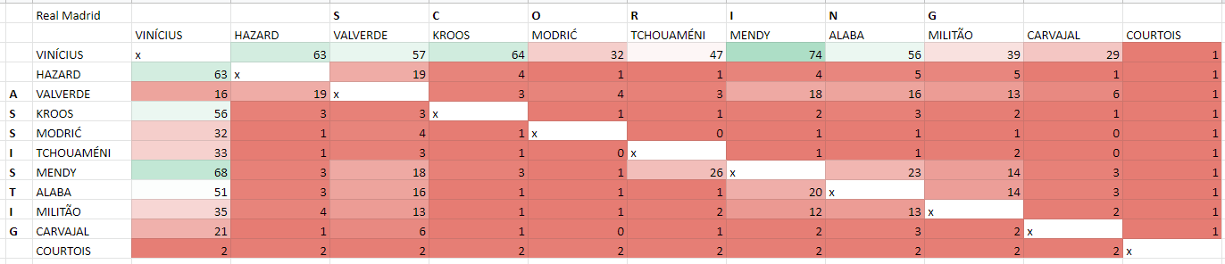
How to read a FBM chart

Maybe you have come across a FBM chart like the following on Twitter and you are curious how to read these charts:

What you see is the answer to the following three questions:

  1. What is the probability that this player is able to contribute to the finishing of his current team?
  2. What is the probability that this player is able to contribute to the defending of his current team?
  3. What is the probability that this player is able to contribute to the passing game of his current team?

These probabilities are predictive and hold for the next upcoming game. It is important to note that almost all statistics in football are backward looking and descriptive. As useful as that can be, descriptive statistics is way less useful than predictive statistics like these FBM stats. After the game these FBM probabilities are updated using Bayes Theorem. For reliable players these probabilities are consistent over time. For more unreliable players they fluctuate more. So you can use FBM statistics to determine how reliable a player is.

Finishing consists of scoring goals, giving assists and shooting on target. The probability of being able to contribute to the finishing of the current team decreases due to shots off target.

Defending consists of all actions of the player and results where the player has a contribution to said result while the opposing team is in possession of the ball. The most positive result is of course gaining possession of the ball.  The probability of being able to contribute to the defending of the current team decreases due to the opposing team getting significantly closer to the goal, fouls being made or goals scored against the team.

Passing game consists of all actions of the player and results where the player has a contribution to said result while the team is in possession of the ball. This includes actions without the ball like drawing out defenders or occupying space, progressive passing, packing and the pre-assist. The probability of being able to contribute to the passing game of the current team decreases due to losing possession of the ball.

Please note that these FBM stats are for playing in their current specific team in their current specific league. We have a Bayesian transfer model to transfer players virtually to different teams and different league. All these probabilities are then adjusted for the new team and in case of a new league also for the new league.

The distribution of probability

The graphs you see are the Poisson distribution of the underlying FBM stats for finishing, defending and passing game. Whenever you see a football statistic given as a single number be very suspicious. Reality is too complex to be captured in numbers, even if there are a whole bunch of them. In fact, the more different statistics are used, the less valuable the information becomes, because the more data you have the more you can prove. Yet, the more you can prove, the more what you prove is confirmation bias as you are going to prove what you already think you know. That is the reason why statistics should now and then shock you. Because if statistics doesn’t shock, the chance is that you use statistics to confirm your biases.

So rather than present players in single numbers, we present players as a Poisson distribution. The distribution gives you the area where the player’s probabilities will lie after the next match. Of course, given that each match only slightly moves these probabilities, if they move at all, in practice these probabilities hold for the whole season or to whenever a major change occurs, like for instance an injury, a new manager or a new team.

A new team is important, because FBM probabilities are always for a player playing for a specific team in a specific league. As soon as the player moves to a different team or even a different league, these probabilities change. We have a Bayesian transfer model that calculates how these probabilities change whenever you move a player from one team to another. Most of what we do is help clubs understand how likely it is that a potential player they like to hire is going to do well in their team.

How to read these distributions

There is a very simple rule to reading these charts:

The more to the right, the better. Ignore the peaks.

Somehow our attention is being drawn to the peaks, but the peaks are a mathematical artifact of the Poisson distribution. You could say that the Poisson distribution tries to distribute 100 points around the average of the statistics. The less space the Poisson distribution has to achieve this, the higher the peak. But the less space means that the probabilities used are very low. Hence the rule to ignore the peaks and just look for what is most to the right. If you really want to know what the vertical values are: the vertical values are the probability of single column in the graph.

Graphs may overlap, so for instance in our example of Oscar Fraulo, he both maxed out on finishing and passing game probabilities and so they overlap turning the graph into some greenish blueish color to indicate that both the green and the blue chart overlap.

If we compare two players in a chart the overlapping area is quite important. Because then the overlapping area is actually the chance that the lesser player will do as good as the better player or even better! So if the graphs of two players overlap a lot, the lesser player has a decent chance of outperforming the better player in the future. Nevertheless, the better player still has the biggest chance of outperforming the lesser player.

When you want to see how one of your favorite players looks in FBM stats, please let us know on Twitter through a Tweet or a DM. Or fill in the form below to request a free sample report:

We respect your email privacy

What is FBM replacement value?

With FBM replacement value we calculate what a club is to be expected to pay minimally to replace one of their players. This calculation is based on the following stats:

  1. The FBM players stats. There are four FBM players stats:
    1. The probability to be able to contribute to the team overall.
    2. The probability to be able to contribute to the finishing of the team.
    3. The probability to be able to contribute to the passing game of the team.
    4. The probability to be able to contribute to the defense of the team.
  2. The historical transfer fees actually paid for the position of the player in the current league.
  3. The rank of the team in the table.
  4. The player’s age.
  5. The player’s length.
  6. The player’s international status.

Replacement value calculates the amount of money a club probably needs to spend to get a replacement player coming to the club. That means that replacement value is more about the new player coming to the club then the player leaving the club. So replacement value is not the most likely transfer fee, but can be used to determine a fair transfer fee by the selling or buying club, or both. That is the reason why replacement fees at some clubs are so much lower than expected transfer fees. These are smart clubs that hire new players for low transfer fees and let them go for high transfer fees. So for example Jurrien Timber of Ajax is expected to leave the club for a transfer fee of thirty million euro. Yet, his replacement value is “only” ten million euro. Yet, this is the amount Ajax needs to spend to get a player back who will produce the same stats as Jurrien Timber.

The way the calculation works is that we start with the perfect player. The FBM player stats are created by using Bayesian statistics. The highest possible probability to be able to contribute is 100%. That means that the perfect player has 100% probability to be able to contribute to the team overall, 100% probability to be able to contribute the finishing of the team, 100% probability to be able to contribute to the passing game of the team, 100% probability to be able to contribute to the defense of the team. Furthermore, the perfect player also has the perfect age and perfect length based on the length and age that have historically gotten the highest transfer fees. The perfect player also plays for the #1 ranked team in the league and he plays for the national team.

Such a player has never yet existed. Even Messi, who scores 100% probability to contribute to the team overall, in finishing and in passing game for most of his career, had a low probability of being able to contribute to the defense of the team.

Nevertheless, even though the perfect player has never existed, we take it that if he did exist, a club should have paid the all time highest transfer fee for that particular position in that particular league for him. In other words, the all time transfer fee actually being paid is to be taken to be paid for the perfect player even if in reality it was not. We don’t want to extrapolate based on the highest fee ever paid, because that fee might be a market top. 

The next step is to check how long ago this top transfer fee was paid and what has happened to the transfer fees paid for that particular position in that particular league. We do this because the market might have topped and we have to take into account that transfer fees in the future go down. This gives us the top transfer fee for the perfect player in the current season.

Finally we calculate how different the actual player is from the perfect player and this gives us the ratio between the actual player and the perfect player. The replacement value is calculated using this ratio and the top transfer fee for the perfect player for that particular position in that particular league.

How replacement value works for clubs and agents

Replacement value is not the most likely transfer fee. The transfer fee is whatever clubs and agents can get away with. Replacement value helps clubs and agents in their negotiations though. Because if club A pays club B a transfer fee that is above the replacement value of the player for club A, then club A is being weakened as the overpay and now have less money available for other transfers. The same goes the other way: if club B sells a player for less than the replacement value of the player for club B, club B is being weakened because they got too little money for the player and have less money left to spend on a replacement or for other players.

Fortunately, this means that it is possible that a transfer is a win/win for both clubs. This is due to the fact that replacement values are specific for each and every club. Player valuations like those on TransferMarkt suggest that the player has an intrinsic worth. This is a statistical mistake. The player only has a value to a specific club. If no club wants a certain player, no matter how high that player is valued, his future transfer fee is zero. So player valuation always needs to be made in the light of the club he is currently playing for and the club he is going to play for, including possible differences in leagues and the rank in the league of both clubs. That means that it is possible, even quite common, that the transfer fee is higher than the replacement value of the player for the club selling the player and at the same time lower than the replacement value of the player for the club buying the player. Both clubs are strengthened by the deal and it is a win/win situation.

Of course, in more cases one club profits at the expense of another club. In that case in very real terms (i.e. money) one club is getting stronger and the other club is getting weaker. So it is very important for clubs to keep checking whether their deals are favorable or not, in the light of the replacement value of the player.

To give an example of how this worked out in practice, we advised one of the consultants working for Willem II in regard to the transfer of Fran Sol to Dinamo Kiev. According to TransferMarkt the value of Fran Sol was 6 million euro at the time. Willem II was trying to get this amount from Dinamo Kiev, but Dinamo Kiev was unwilling to pay this amount. In our calculations Fran Sol had a replacement value of only 2 million for Willem II and 4 million for Dinamo Kiev. So any amount between 2 million and 4 million would be a win/win for both clubs. The final deal was for 3.5 million euro.

Given that the player’s age is a factor in the calculation of the replacement value, one can easily calculate the replacement value of a player in the future. This way clubs and agents can see whether a potential transfer has the chance of being profitable if the player leaves his new club after one or two seasons. That is how we were able to predict that Dalmau, who came to Heracles as a free agent, would have a replacement value of 1.75 million euro one season later. Indeed, after one season playing for Heracles he was transferred to FC Utrecht for 700.000 euro plus the transfer of Dessers to Heracles. Dessers at the time was valued at 1 million euro, bringing the value of the complete deal to 1.7 million euro, very close to the replacement value of 1.75 million euro we predicted for Heracles. Dessers left Heracles also after playing there for just one season for a 4 million euro transfer fee.

Why there, sometimes, is a big gap between FBM replacement value and transfer fees valuations

Take the interesting case of Noussair Mazraoui

His replacement value is 6.5 million euro playing for Ajax in the Eredivisie. Yet, his valuation at TransferMarkt is 20 million euro. Noussair Mazraoui is leaving as a free agent, so we will never know what the transfer fee would have been, but it doesn’t seem that Ajax has gotten a very attractive offer for Noussair Mazraoui. 

Nevertheless, there is a big gap between 6.5 million and 20 million. This gap is a great example of why replacement value is not the same as transfer fees. The FBM replacement value is a measure for Ajax to limit their spending on a replacement for Noussair Mazraoui to 6.5 million euro. We might be mistaken, but we think it is highly unlikely that Ajax would spend more than 6.5 million euro. Cases like these validate the replacement value model.

Some superstar players have extremely high valuation on sites like TransferMarkt. Mainly because they play in one of the best leagues for some of the best clubs, often getting very far in the Champions League. These high valuation are more a token of appreciation than a likely transfer fee as most of these superstar players will stay with their current club until (almost) the end of their career. Without the prospect of a transfer, the real value of those players is much closer to zero than the extremely high number quoted everywhere. So once more clubs find more use in the replacement value of those players as at some point they have to replace their retiring superstars with other players.

Even though FBM replacement values are not meant to predict future transfer fees, in 2 out of 3 cases FBM replacement values are closer to the actual transfer fees than the valuation at TransferMarkt.

Undervalued players

Even though replacement value is really about the next player coming in to replace the current player, if the replacement value is much higher than the actual valuation, then one still can say that they player is undervalued. The reason being that if the club were to sell their current player for the valuation fee and then had to hire a new player for the much higher replacement value, they would lose a lot of money. Hence players whose replacement value is much higher than their public valuation are undervalued. Here is a list of some of the undervalued players we have found.